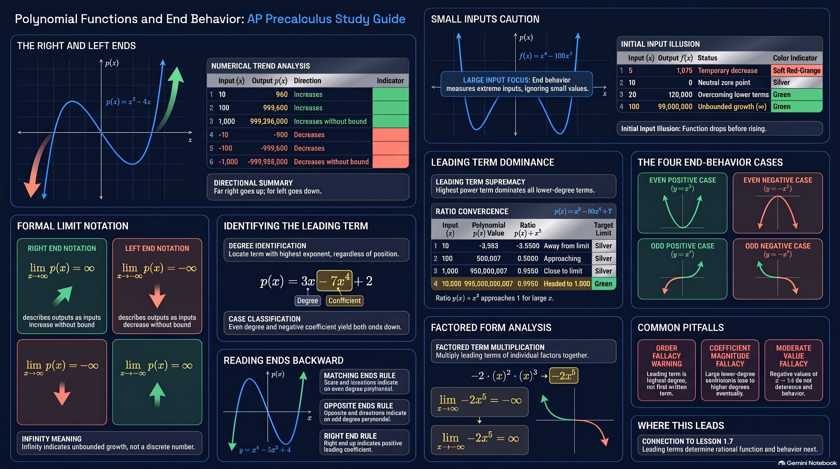
Use this as a quick reference for limit notation at both ends, the leading term dominating, the four end-behavior patterns, and reading ends from graphs.
🧭 Plot Summary
Lesson 1.5 found where a polynomial hits zero. Now zoom all the way out. As x increases or decreases without bound, the outputs of a nonconstant polynomial either increase or decrease without bound, and you write that with limit notation such as limx→∞ p(x) = ∞. The reason is that the leading term dominates every lower-degree term once the inputs are large. So just two facts decide both ends: whether the degree is even or odd, and whether the leading coefficient is positive or negative.
What you'll do in this lesson
Describe what a nonconstant polynomial does as x increases without bound.
Describe what it does as x decreases without bound, using limit notation.
Explain why the leading term dominates the lower-degree terms.
Use the degree and the sign of the leading term to predict both ends.
Find the leading term from a factored form without multiplying out.
Read end behavior from a graph and work backward to the degree and sign.
Why it matters
Long-run behavior is the question behind every model: where does the population, the cost, or the height go if the model keeps running? The ends tell you whether a polynomial model can be trusted far from the data. Lesson 1.7 uses the same dominance idea on a quotient of two polynomials.
✅ Self-Check Before You Move On
Check off each item as you get there. These aren't grades — they're your own signal.