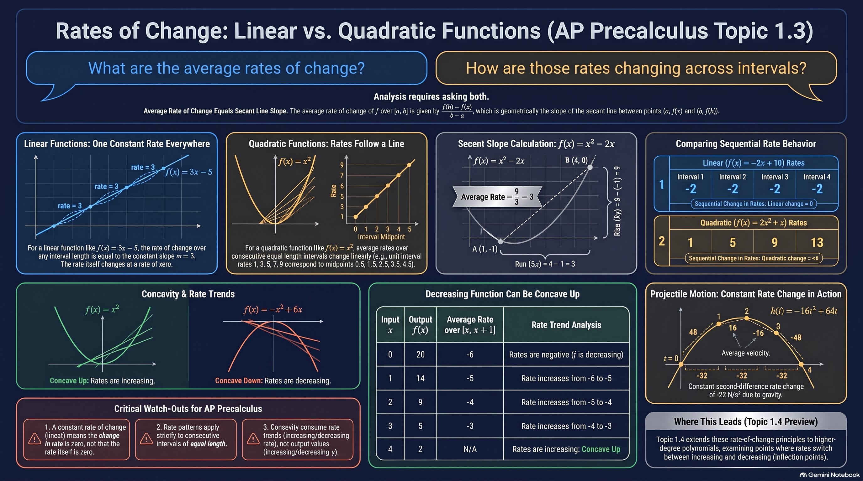
Use this as a quick reference for linear and quadratic rates of change, secant slopes, how fast the rates are changing, and concavity.
🧭 Plot Summary
Lesson 1.2 taught you to measure how fast a function changes. Now you meet the two most important families. A linear function has the same average rate of change over every interval, so its rates are changing at a rate of zero. A quadratic function has rates that depend on where you look, but over consecutive equal-length intervals they follow a linear function, so they change at a constant rate. Each average rate is the slope of a secant line, and when the rates are increasing the graph is concave up, when they are decreasing it is concave down.
What you'll do in this lesson
Show that a linear function has one constant average rate of change on every interval.
Find the average rates of a quadratic over consecutive equal-length intervals and see that they follow a line.
Read the average rate of change as the slope of a secant line.
Measure how fast the average rates are changing: zero for linear, constant for quadratic.
Use increasing and decreasing rates to decide concave up and concave down.
Decide from a table whether data is linear, quadratic, or neither.
Why it matters
Projectile motion, break-even profit, and area models are all quadratic. Knowing that their rates change steadily is what lets you predict the next value from a table, spot a quadratic model, and explain the shape of a graph. It also sets up polynomial rates in Lesson 1.4 and, later, the idea of the derivative.
✅ Self-Check Before You Move On
Check off each item as you get there. These aren't grades — they're your own signal.