Angular Momentum and Angular Impulse

🧭 Plot Summary

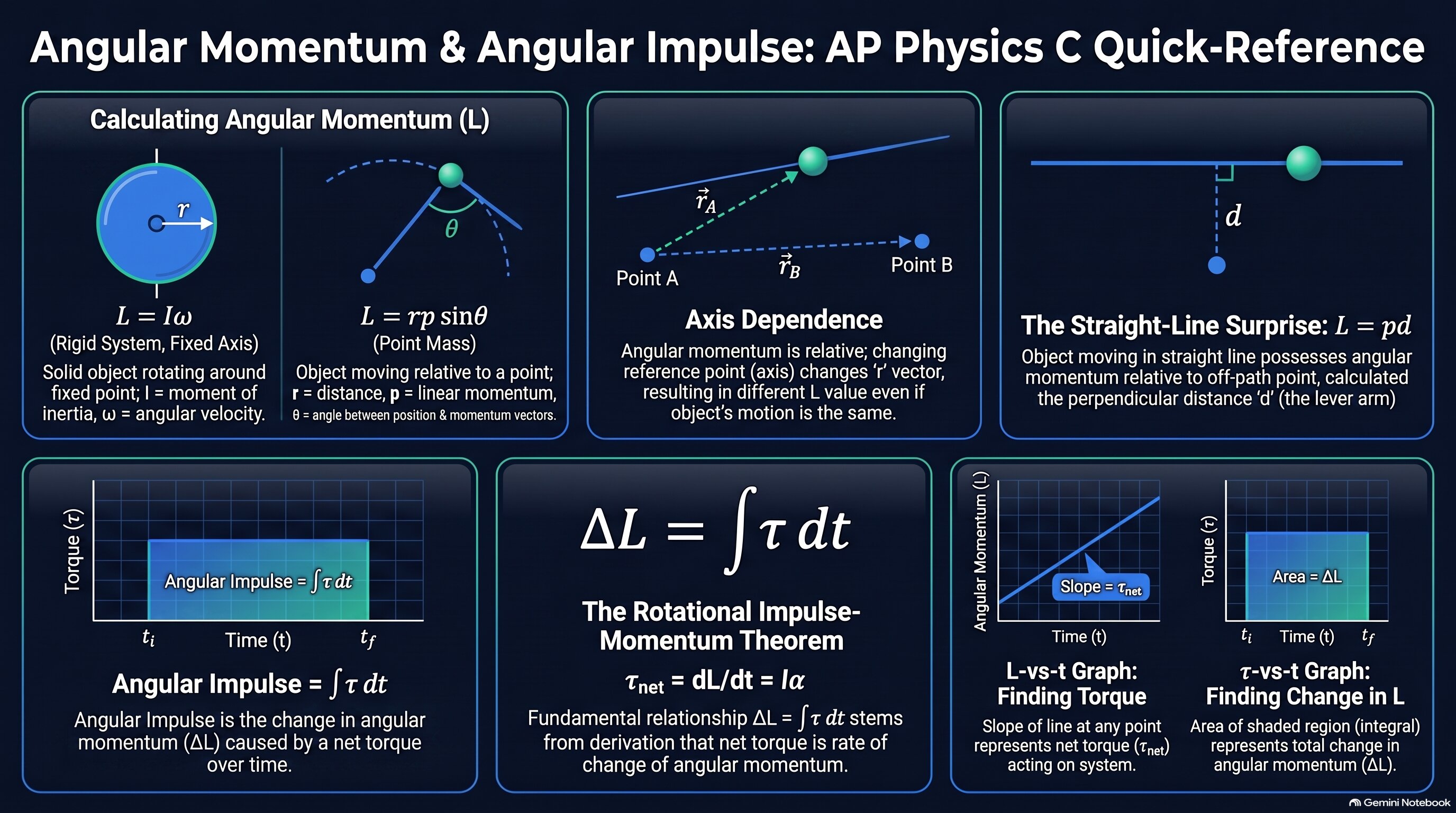
Back in Unit 4, linear momentum (p⃗ = mv⃗) gave you a way to track translational motion through collisions and explosions. This lesson introduces its rotational counterpart: angular momentum. For a rigid system spinning about a fixed axis, it's simply L = Iω. But angular momentum is more general than that — any object, even one moving in a perfectly straight line, has an angular momentum about a chosen point, given by L = rp sinθ. On the impulse side, a torque sustained over a time interval delivers an angular impulse, and — just like the linear impulse–momentum theorem from Unit 4 — that angular impulse equals the resulting change in angular momentum: ΔL = ∫τ dt.

What you'll do in this lesson

• Calculate the angular momentum of a rigid system rotating about a fixed axis using L = Iω.
• Calculate the angular momentum of any object about a point using L = rp sinθ, even objects moving in a straight line.
• Recognize that angular momentum depends on the axis or point it's measured about.
• Calculate angular impulse from a torque using ∫τ dt, or from the area under a torque-vs-time graph.
• Apply the rotational impulse-momentum theorem: angular impulse equals the change in angular momentum.
• Read net torque directly off the slope of an angular-momentum-vs-time graph.

Why it matters

This lesson builds the exact toolkit Lesson 6.4 needs: once you can find an object's angular momentum and track how torques change it, conservation of angular momentum — what happens when the net external torque is zero — is a short step away.

✅ Self-Check Before You Roll On

Check off each item as you get there. These aren't grades — they're your own signal.