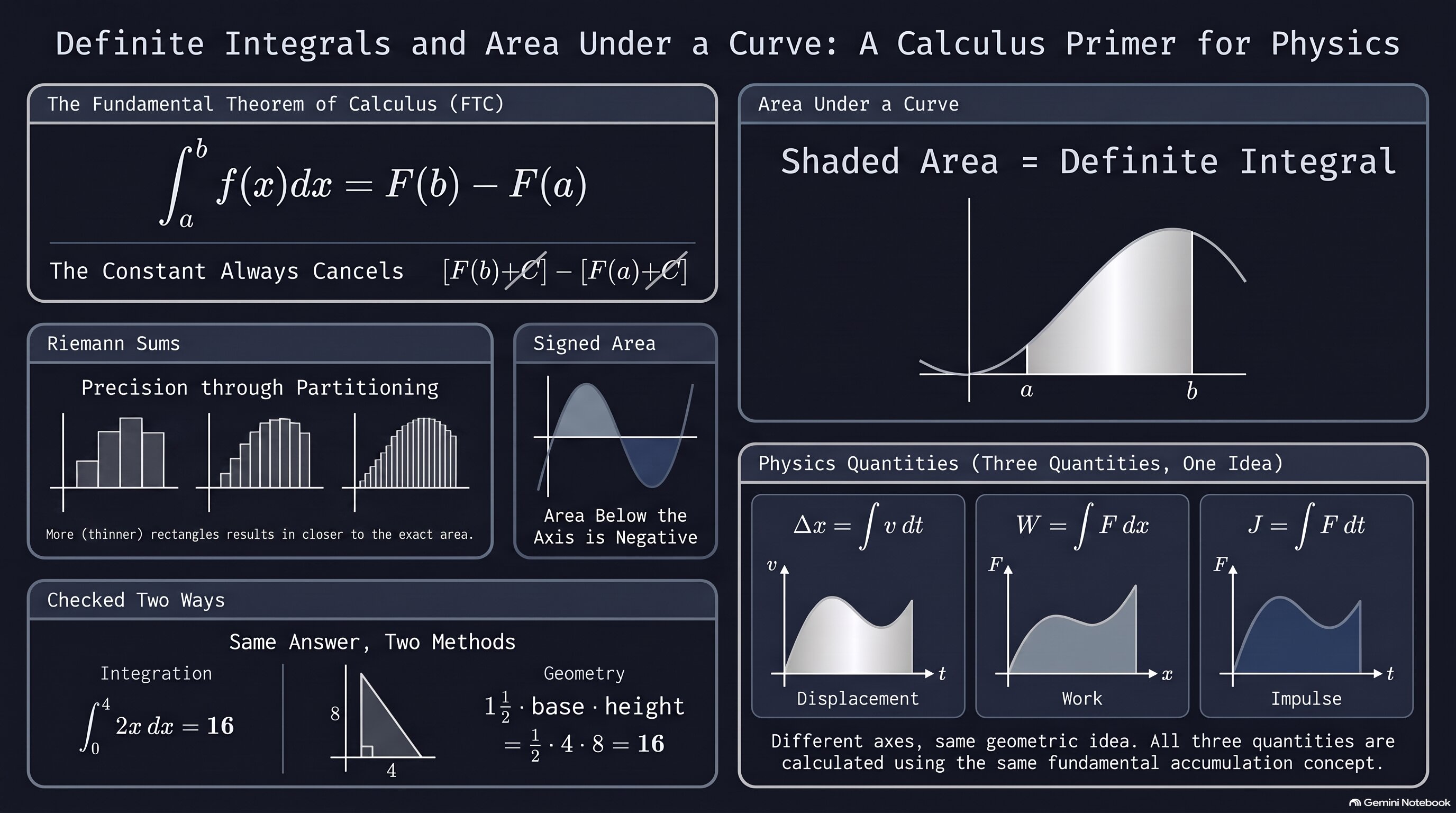
Use this as a quick reference for the Fundamental Theorem of Calculus, Riemann sums, and the "area under the curve" pattern that shows up across the whole course.
🧭 Plot Summary
Lesson 0.4 found families of antiderivatives, each one still missing a specific constant. This lesson closes that gap by asking a slightly different question: what if you evaluate an antiderivative at two specific points and subtract? That small change turns integration into something concrete — a single number — and that number has a beautiful geometric meaning: it's the area between a curve and the x-axis. This one idea, area under a curve, is the picture hiding behind an enormous number of physics equations you'll meet this year.
What you'll do in this lesson
- State and apply the Fundamental Theorem of Calculus.
- See why the constant of integration disappears in a definite integral.
- Interpret a definite integral geometrically as signed area under a curve.
- Watch a Riemann sum converge to an exact area as rectangles get thinner.
- Check a definite integral's value against a geometric area calculation.
- Compute displacement, work, and impulse — all as area under a curve.
Why it matters
Δx = ∫v dt, W = ∫F dx, and J = ∫F dt look like three unrelated formulas from three different units. They're the same idea, three times: displacement is the area under a velocity-time graph, work is the area under a force-position graph, and impulse is the area under a force-time graph.
✅ Self-Check Before You Roll On
Check off each item as you get there. These aren't grades — they're your own signal.